Intraday Trading Algorithm for Energy Storage Systems
Linear programming approaches and rolling horizons. A dynamic algorithm for intraday energy trading.
This post documents my experience applying data science to algorithmic trading in energy storage systems.
The goal is to develop an algorithm that maximizes profit by strategically buying energy during low market prices and selling at peak times. It must estimate cycle costs while adhering to the following constraints:
- Nominal power: 2 MW
- Usable capacity: 4 MWh
- Storage efficiency: 90%
- Target average cycles per 24-hour horizon: 1.5
- Maximum cycles per 24-hour horizon: 2.5
The theoretical background is available of my GitHub and explains each of the basic constraints and the dynamics of energy storage systems.
With that out of the way, let’s get to it!
Solution
First things first, importing the necessary libraries:
# Importing necessary libraries for this project

import numpy as np
import pandas as pd
import matplotlib.pyplot as plt
import seaborn as sns
from itertools import combinations
from scipy.optimize import linprog
# Import data
market_prices_df = pd.read_csv(r"market_prices.csv", sep=';', parse_dates=['timestamp_UTC'])
market_prices_df.info()
<class 'pandas.core.frame.DataFrame'>
RangeIndex: 35040 entries, 0 to 35039
Data columns (total 2 columns):
 #   Column                                Non-Null Count  Dtype
---  ------                                --------------  -----
 0   timestamp_UTC                         35040 non-null  datetime64[ns]
 1   price_idm_continuous_qh_vwap_EUR/MWh  35040 non-null  float64
dtypes: datetime64[ns](1), float64(1)
memory usage: 547.6 KB
The raw data contains 35,040 observations (15-minute intervals) of MWh prices in euros. We transform and group this into 366 days with 96 observations each to simplify analysis. We also define our system constraints.
market_prices_df = market_prices_df.rename(columns={market_prices_df.columns[1]: 'EUR/MWh'})
market_prices_df['date'] = market_prices_df['timestamp_UTC'].dt.date
daily_price_data = market_prices_df.groupby('date')['EUR/MWh'].apply(list).reset_index()
daily_price_data.head()
<class 'pandas.core.frame.DataFrame'>
RangeIndex: 366 entries, 0 to 365
Data columns (total 3 columns):
 #   Column      Non-Null Count  Dtype
---  ------      --------------  -----
 0   date        366 non-null    object
 1   EUR/MWh     366 non-null    object
 2   cycle_cost  366 non-null    float64
dtypes: float64(1), object(2)
memory usage: 8.7+ KB
After transforming the data into neat 366 days with 96 observations aggregated into a list for each day, the data becomes much easier to work with. Before going on to our solution, we set the constraints early on in the project
#Constraints:
nominal = 2  # in MW
capacity = 4  # in MWh
efficiency = 90 / 100  # 90%
target_average_cycles = 1.5
max_cycles_per_day = 2.5
1. The Combinatory Approach
The initial algorithm consists of two components: cycle calculation and cost estimation.
1. Determining best trading cycles in the day
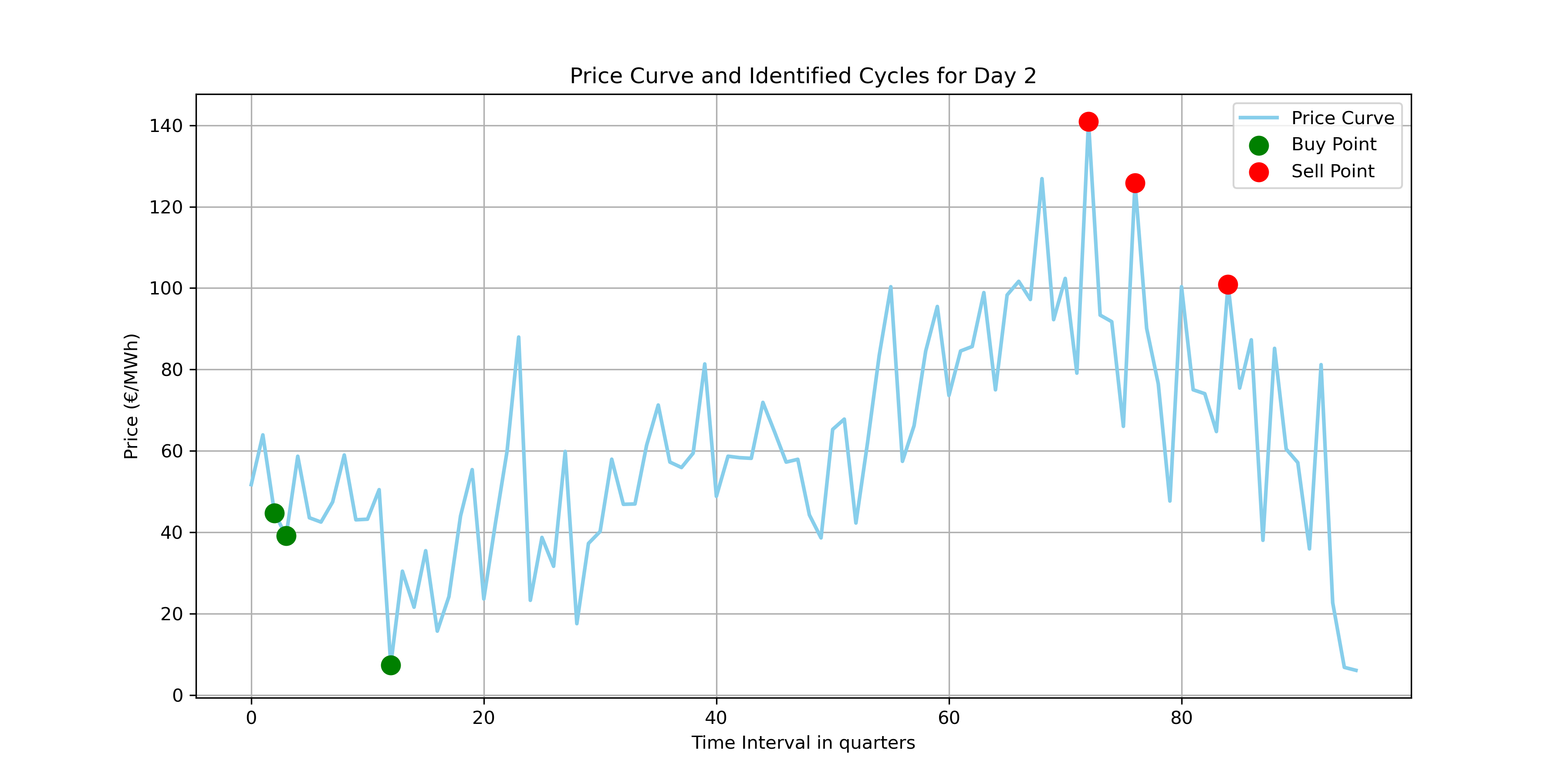
calculate_daily_cycles identifies the most profitable daily transactions based on the expected spread (selling price minus buying price, adjusted for efficiency). It calculates all possible spreads, sorts them by descending profitability, and limits them within operational bounds.
#Define a function to calculate the daily cycles with most the spread, while considering storage limitations and efficiency.

def calculate_daily_cycles(price_data):
    num_intervals = len(price_data)
    best_spreads = []

    for buy_time, sell_time in combinations(range(num_intervals), 2):
        spread = (price_data[sell_time] * efficiency * efficiency)
        - price_data[buy_time]
        best_spreads.append((spread, buy_time, sell_time))

    best_spreads.sort(reverse=True)
The function tracks used intervals to avoid overlaps, computes the exact energy amounts (bought, charged, discharged), calculates profit, and halting once the maximum daily cycles limit is reached.
cycles = []
used_intervals = set() #used instead of empty list for faster lookup time of if statment
for spread, buy_time, sell_time in best_spreads:
    if buy_time not in used_intervals and sell_time not in used_intervals:
        required_input_energy = capacity / efficiency #Energy required to buy to fill up the battery's capacity
        bought_energy = min(nominal * (sell_time - buy_time) * 0.25, required_input_energy)
        charged_energy = bought_energy * efficiency
        discharge_energy = charged_energy * efficiency
        profit = price_data[sell_time]*discharge_energy - price_data[buy_time]*bought_energy

        cycles.append({
            'buy_time': buy_time,
            'sell_time': sell_time,
            'bought_energy':bought_energy,
            'charged_energy': charged_energy,
            'discharge_energy': discharge_energy,
            'buy_price': price_data[buy_time],
            'sell_price': price_data[sell_time],
            'spread': f'{round(spread, 2)} EUR',
            'profit': f'{round(profit, 2)} EUR' ,
        })

        used_intervals.update(range(buy_time, sell_time + 1))

        if len(cycles) >= max_cycles_per_day:
            break

return cycles

# Test the function with data for one day
test_day_data = daily_price_data['EUR/MWh'].iloc[1]
calculate_daily_cycles(test_day_data)
2. Estimate the cost of cycles
estimate_cycle_costs computes the net cost per unit of energy cycled based on the purchased input energy. By tallying total purchase cost minus total sales revenue, a negative net cost signifies profit.
def estimate_cycle_costs(cycles):
    total_purchase_cost = 0
    total_sales_revenue = 0
    total_energy_cycled = 0

    for cycle in cycles:
        total_purchase_cost += cycle['bought_energy'] * cycle['buy_price']
        total_sales_revenue += cycle['discharge_energy'] * cycle['sell_price']
        total_energy_cycled += cycle['bought_energy'] #Bought energy is used to represents a complete energy cycle as it was the intial input energy

    net_cost = total_purchase_cost - total_sales_revenue
    cycle_cost = net_cost / total_energy_cycled

    return cycle_cost

test_day_cycles = calculate_daily_cycles(daily_price_data['EUR/MWh'].iloc[1])
estimate_cycle_costs(test_day_cycles)
Visualizing the buy and sell times, we confirm the algorithm correctly selects profitable cycles.
3. Visualizing results
Comparing the cycle costs applied to the first 10 days arrayed below:
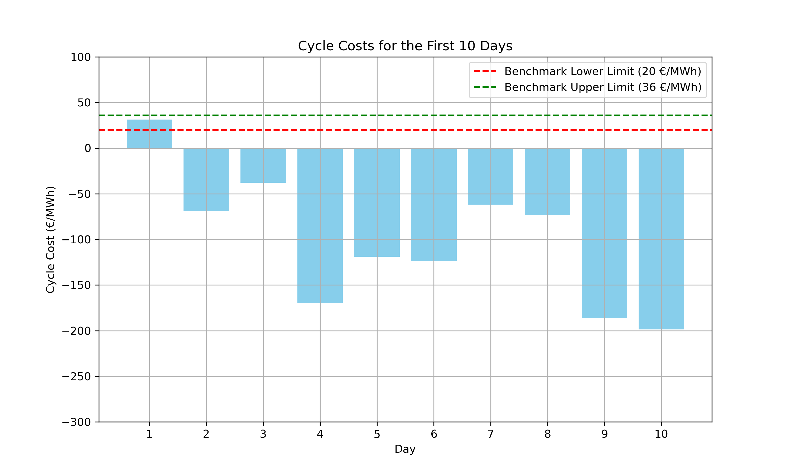
print(f"{((daily_price_data['cycle_cost'] >= 20) & (daily_price_data['cycle_cost'] <= 36)).sum()} day(s) within benchmark.")
Output
1 day(s) within benchmark.The first day yielded costs within our benchmark, but analyzing just four data points suggests a rolling horizon approach—as recommended by the challenge—might be more effective.
2. The Rolling Horizon Approach
Instead of processing an entire day at once, a rolling horizon analyzes a smaller time window and continuously shifts forward by a defined step size, allowing the algorithm to dynamically adapt to recent market prices.
1. Constructing the rolling horizon
def calculate_daily_cycles_rolling_horizonv2(price_data, current_avg_cycles, horizon_length=8, step_size=1):
    num_intervals = len(price_data)
    best_cycles = []

    #Dynamically change max number of cycles per day based on the target and current average number of cycles
    max_cycles_per_day = min(2.5, max(1, target_average_cycles + (target_average_cycles - current_avg_cycles)))
I dynamically adjust the maximum daily cycles based on the gap between the target and current average, helping the algorithm align with long-term goals.
 # Loop over data with the rolling horizon
    for start_time in range(0, num_intervals, step_size):
        end_time = min(start_time + horizon_length, num_intervals)
        best_spreads = []
    return best_cycles
A loop shifts the rolling window forward by step_size. For each window, it searches for profitable cycles using the same combinatory logic but calculates against the modulated cycle allowance max.
current_avg_cycles = 0
num_days = len(daily_price_data)

for i in range(num_days):
    daily_data = daily_price_data['EUR/MWh'].iloc[i]
    cycles = calculate_daily_cycles_rolling_horizonv2(daily_data, current_avg_cycles)
    cycle_cost = estimate_cycle_costs(cycles)
    daily_price_data.at[i, 'cycle_cost'] = cycle_cost
    current_avg_cycles = ((current_avg_cycles * i) + len(cycles)) / (i + 1)
Iterating through the entire dataset, we update the rolling average cycle count continuously, ensuring each cycle assessment remains responsive to up-to-date data.
2. Identifying the best parameters
To optimize the strategy, we tested various horizon lengths and step sizes to maximize the number of days meeting our benchmark cycle costs.
#Trying out different parameters
results = []

for horizon_length in [4, 8, 12, 16, 20, 24, 28, 32]:
    for step_size in [1, 2, 4, 6, 8, 10]:
        daily_cycle_costs = daily_price_data['EUR/MWh'].apply(
            lambda x: estimate_cycle_costs(calculate_daily_cycles_rolling_horizon(x, horizon_length=horizon_length, step_size=step_size))
        )
        results.append({
            'horizon_length': horizon_length,
            'step_size': step_size,
            'days_within_benchmark': ((daily_cycle_costs >= 20) & (daily_cycle_costs <= 36)).sum()
        })

results_df = pd.DataFrame(results)
results_df.sort_values(by='days_within_benchmark',ascending=False).head()
Output
| horizon_length | step_size | days_within_benchmark |
|---|---|---|
| 8 | 1 | 90 |
| 8 | 2 | 90 |
| 8 | 4 | 89 |
| 8 | 6 | 89 |
| 8 | 10 | 89 |
The code iterates over a predefined set of horizon lengths and step sizes, applying each combination to the daily price data. For each set of parameters, it calculates the cycle costs for each day and then aggregates the number of days where the cycle cost falls within the benchmark range. With the horizon length of two hours and step sizes of 1 and 2 yielding the highest results, respectively.
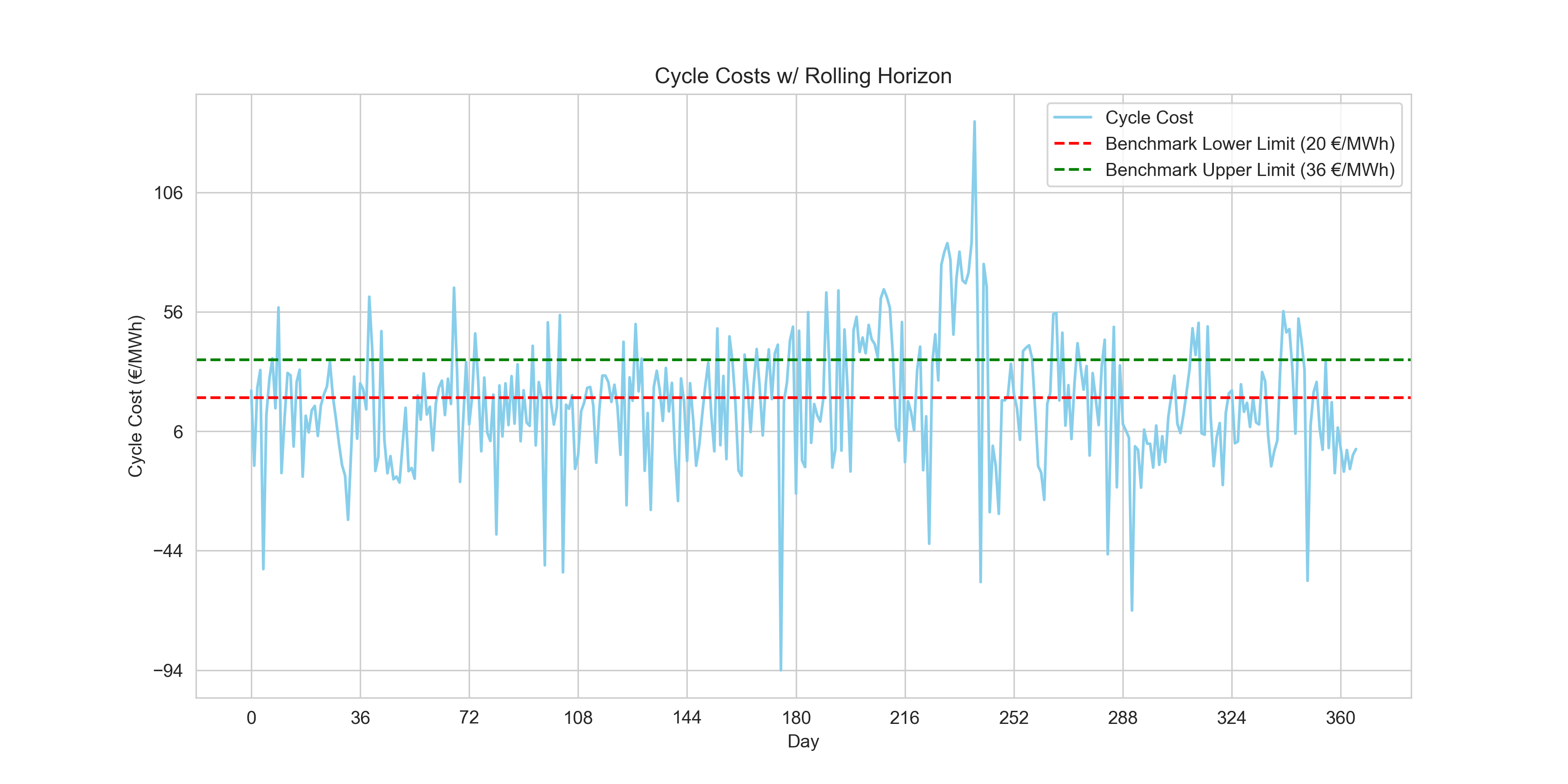
3. 89 new observations within benchmarks
plt.figure(figsize=(12, 6))

plt.plot(daily_price_data.index, daily_price_data['cycle_cost'], color='skyblue', label='Cycle Cost')
plt.axhline(y=20, color='r', linestyle='--', label='Benchmark Lower Limit (20 €/MWh)')
plt.axhline(y=36, color='g', linestyle='--', label='Benchmark Upper Limit (36 €/MWh)')
plt.xlabel('Day')
plt.ylabel('Cycle Cost (€/MWh)')
plt.title('Cycle Costs w/ Rolling Horizon')
plt.legend()
plt.grid(True)
plt.xticks(range(0, len(daily_price_data['cycle_cost']), int(len(daily_price_data['cycle_cost'])/10)))
plt.yticks(range(int(daily_price_data['cycle_cost'].min()), int(daily_price_data['cycle_cost'].max()), 50))
plt.show()
print(f"{((daily_price_data['cycle_cost'] >= 20) & (daily_price_data['cycle_cost'] <= 36)).sum()} day(s) within benchmark. \nCurrent Average Number of cycles: {round(current_avg_cycles, 3)}")
Output
90 day(s) within benchmark.
Current Average Number of cycles: 1.997
We raised our benchmark-compliant days to 90. However, while the vast majority of our daily cycle costs are strongly negative (demonstrating solid absolute profit), establishing a robust algorithm that cleanly sits within the specific arbitrary positive benchmark range set by this challenge will require a heavier-handed tool.
3. The Constrained Optimization Approach
Upon encountering this obstacle, I had to do some research on how to approach this project as my only data science experience so far was related to machine learning algorithms. On data science forums as I was debating my combinatory rolling horizon approach, it was pointed out to me that perhaps I’d find my answer in a constrained optimization approach. Although ignorant of it at first, I found it extremely fitting to the problem at hand! The approach attempts to identify the best ways to maximize a function within a set of hard and soft constraints. Sounds familiar?
It uses linear programming to maximize our energy trading strategy’s profitability. By utilizing the entire dataset from the outset, the optimization model takes a holistic view of the data, analyzes all these potential cycles collectively and determines the optimal set of cycles that could achieve the maximum possible profit. It compiles all possible trading cycles from the entire dataset of energy prices upfront. Each cycle’s profitability is assessed based on the prices at potential buy and sell times, factoring in the system’s operational constraints such as energy capacity, charging and discharging efficiencies, and the overall number of cycles allowed.
This approach contrasts with a rolling horizon, which would have looked at the data in chunks—optimizing over a short window and then rolling that window forward through the dataset, iteratively recalculating the optimal cycles as new price data becomes available.
Therefore, I chartered out to use a solver that makes use of SciPy, the famous Python package for mathematical computations among other uses.
1. Defining decision variables
First, generate_possible_cycles enumerates all possible daily buying and selling cycles to serve as decision variables. It works identically to our initial combinatory approach but omits sorting or halting at maximum limits.
#Create function to generate all possible cycles for one day, important for defining decision variable.
def generate_possible_cycles(price_data, min_length=1):
    num_intervals = len(price_data)
    possible_cycles = []

    for buy_time, sell_time in combinations(range(num_intervals), 2):
        if sell_time - buy_time >= min_length:
            spread =  (price_data[sell_time] * efficiency * efficiency) - price_data[buy_time]
            required_input_energy = capacity / efficiency
            bought_energy = min(nominal * (sell_time - buy_time) * 0.25, required_input_energy)
            charged_energy = bought_energy * efficiency
            discharge_energy = charged_energy * efficiency
            profit = price_data[sell_time]*discharge_energy -price_data[buy_time]*bought_energy

            possible_cycles.append({
                'buy_time': buy_time,
                'sell_time': sell_time,
                'bought_energy': bought_energy,
                'charged_energy': charged_energy,
                'discharge_energy': discharge_energy,
                'buy_price': price_data[buy_time],
                'sell_price': price_data[sell_time],
                'spread': spread,
                'profit': profit,
            })

    return possible_cycles


sample_day_data = daily_price_data['EUR/MWh'].iloc[1]
sample_possible_cycles = generate_possible_cycles(sample_day_data)
sample_possible_cycles_df = pd.DataFrame(sample_possible_cycles)
sample_possible_cycles_df.head()

#Create function to generate possible cycles for all days
def generate_possible_cycles_for_all_days(daily_price_data, min_length=1):
    all_possible_cycles = []

    for day_index, price_data in enumerate(daily_price_data['EUR/MWh']):
        daily_possible_cycles = generate_possible_cycles(price_data, min_length)

        #add day index to each cycle to identify the day to which it belongs
        for cycle in daily_possible_cycles:
            cycle['day_index'] = day_index

        all_possible_cycles.extend(daily_possible_cycles)

    return all_possible_cycles

all_possible_cycles = generate_possible_cycles_for_all_days(daily_price_data)
all_possible_cycles_df = pd.DataFrame(all_possible_cycles)
all_possible_cycles_df.head(), all_possible_cycles_df.info()
Output
<class 'pandas.core.frame.DataFrame'>
RangeIndex: 1664032 entries, 0 to 1664031
Data columns (total 10 columns):
 #   Column            Non-Null Count    Dtype
---  ------            --------------    -----
 0   buy_time          1664032 non-null  int64
 1   sell_time         1664032 non-null  int64
 2   bought_energy     1664032 non-null  float64
 3   charged_energy    1664032 non-null  float64
 4   discharge_energy  1664032 non-null  float64
 5   buy_price         1664032 non-null  float64
 6   sell_price        1664032 non-null  float64
 7   spread            1664032 non-null  float64
 8   profit            1664032 non-null  float64
 9   day_index         1664032 non-null  int64
dtypes: float64(7), int64(3)
memory usage: 127.0 MB
The results show over 1.66 million possible cycles, ready for constraint filtering.
2. Using linear programming
Linear programming is a powerful tool used in operations research to find the best outcome in a mathematical model whose requirements are represented by linear relationships. In the context of our project, LP will help us identify the most profitable set of cycles that can be executed within the operational constraints of the energy storage system.
We establish our objective function, c, as the negation of the cycle profits (since LP minimizes functions by default). We enforce our cycle limits using matrix A_eq_daily for the daily maximum and A_eq_average for the overall target average.
#Using linear programming
days_number = daily_price_data.shape[0]

profits = all_possible_cycles_df['profit'].values
day_indices = all_possible_cycles_df['day_index'].values
c = -profits
lambda_penalty = 1e6

A_eq_daily = np.zeros((days_number, len(profits)))
for i in range(days_number):
    A_eq_daily[i, day_indices == i] = 1

A_eq_average = np.ones((1, len(profits)))

A_eq = np.vstack([A_eq_daily, A_eq_average])
b_eq = np.hstack([np.full(days_number, max_cycles_per_day), [target_average_cycles * days_number]])

c_extended = np.append(c, lambda_penalty)#Extend c to account for the penalty on the deviation variable delta


A_eq_delta = np.append(np.ones(len(profits)), [-1]).reshape(1, -1)
A_eq = np.hstack([A_eq, np.zeros((A_eq.shape[0], 1))])  # Add a column for delta to A_eq
A_eq[-1, :] = A_eq_delta  # Update the last row with A_eq_delta


bounds = [(0, 1) for _ in profits] + [(0, None)]
print(A_eq.shape, b_eq.shape)
We stack constraints into A_eq and b_eq, imposing a high lambda_penalty on deviations from the target average. The decision bounds are binary (0, 1) to indicate whether a given cycle should be executed, while the penalty deviation variable can adjust freely above zero.
Output
(367, 1664033) (367,)
2.1 Using the solver
res_option_b = linprog(c_extended, A_eq=A_eq, b_eq=b_eq, bounds=bounds, method='highs')
print(res_option_b)
message: Optimization terminated successfully.
            (HiGHS Status 7: Optimal)
success: True
    status: 0
    fun: 365095106.33555603
        x: [ 0.000e+00  0.000e+00 ...  0.000e+00  3.660e+02]
    nit: 375
    lower:  residual: [ 0.000e+00  0.000e+00 ...  0.000e+00
                        3.660e+02]
            marginals: [ 1.707e+01  4.832e+01 ...  1.425e+02
                        0.000e+00]
    upper:  residual: [ 1.000e+00  1.000e+00 ...  1.000e+00
                            inf]
            marginals: [ 0.000e+00  0.000e+00 ...  0.000e+00
                        0.000e+00]
    eqlin:  residual: [ 0.000e+00  0.000e+00 ...  0.000e+00
                        0.000e+00]
            marginals: [ 1.000e+06  9.996e+05 ...  9.999e+05
                        -1.000e+06]
ineqlin:  residual: []
            marginals: []
 mip_node_count: 0
 mip_dual_bound: 0.0
        mip_gap: 0.0
The solver outputs the optimal objective function value (fun), representing maximized profit, and returns binary execution choices X for each potential cycle. The mip_gap of 0 confirms an optimal solution.
x_values = res_option_b['x'][:-1]
suggested_cycle_indexes = np.where(x_values == 1)[0]
suggested_cycles_df = all_possible_cycles_df.iloc[suggested_cycle_indexes]
suggested_cycles_df
We reconstruct the selected cycles into suggested_cycles_df by filtering all_possible_cycles_df for rows where the x_values binary decision is 1, leaving us with the exact operations suggested by the LP model.
suggested_df = suggested_cycles_df.groupby('day_index').apply(lambda x: x.to_dict('records'))Cycles are grouped by day to format seamlessly into our estimate_cycle_costs reporting function.
3. Visualizing the suggested cycles
#Plotting out final cycle cost estimations using the suggest cycles of the linear programming method.
daily_price_data['cycle_cost'] = suggested_df.apply(estimate_cycle_costs)
plt.figure(figsize=(12, 6))
plt.plot(daily_price_data.index, daily_price_data['cycle_cost'], color='skyblue', label='Cycle Cost')
plt.axhline(y=20, color='r', linestyle='--', label='Benchmark Lower Limit (20 €/MWh)')
plt.axhline(y=36, color='g', linestyle='--', label='Benchmark Upper Limit (36 €/MWh)')
plt.xlabel('Day')
plt.ylabel('Cycle Cost (€/MWh)')
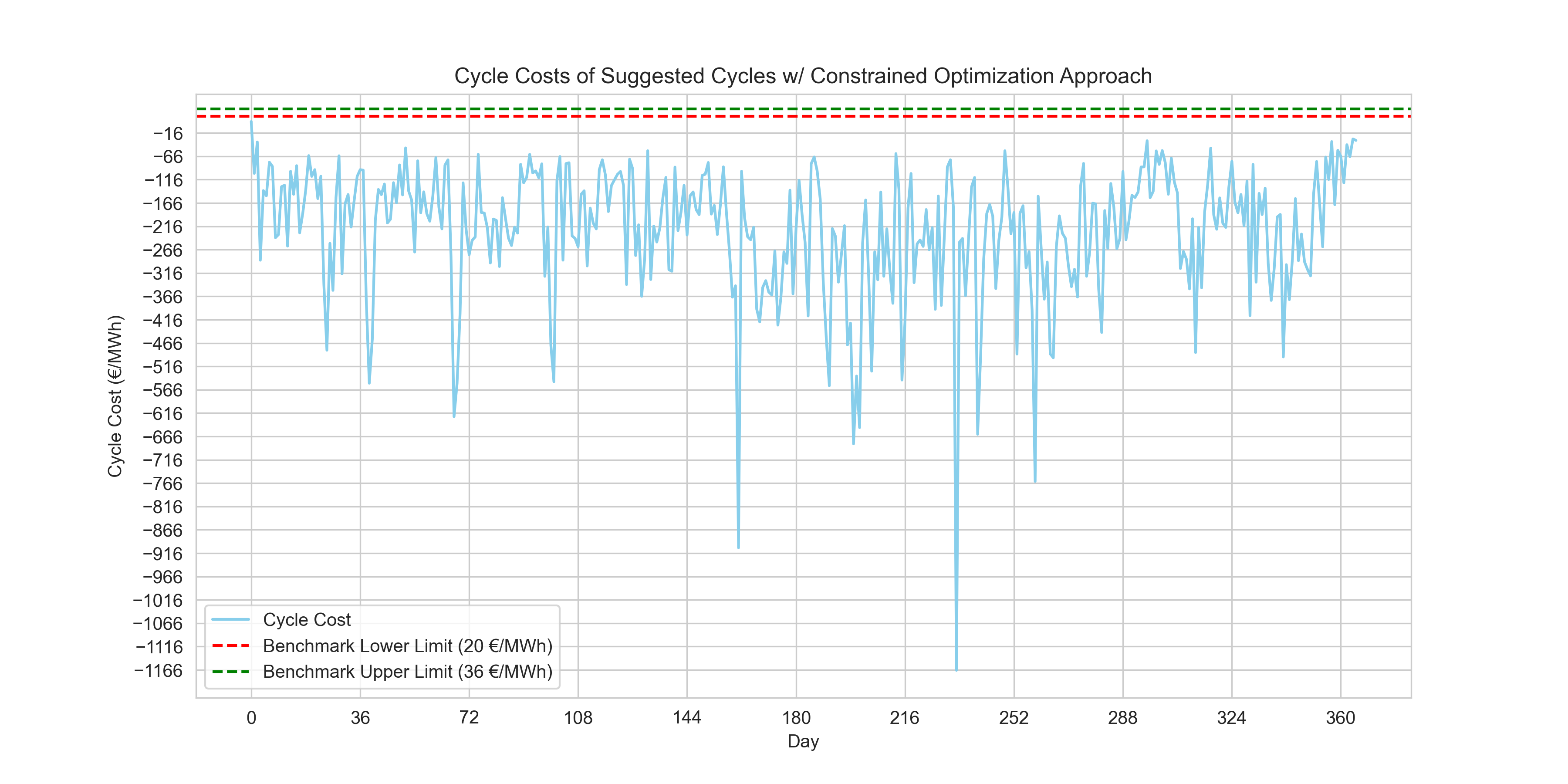
plt.title('Cycle Costs of Suggested Cycles w/ Constrained Optimization Approach')
plt.legend()
plt.grid(True)
plt.xticks(range(0, len(daily_price_data['cycle_cost']), int(len(daily_price_data['cycle_cost'])/10)))
plt.yticks(range(int(daily_price_data['cycle_cost'].min()), int(daily_price_data['cycle_cost'].max()), 50))
plt.show()
print(f"{((daily_price_data['cycle_cost'] >= 20) & (daily_price_data['cycle_cost'] <= 36)).sum()} day(s) within benchmark.")
Output
0 day(s) within benchmark.Conclusion
Our LP optimization yielded purely zero days within the challenge benchmark limits. However, those specific positive benchmarks remain oddly counterintuitive when the ultimate purpose in trading evaluation is profit generation (a strongly negative net cost).
If we strictly evaluate total profit maximization instead of the benchmark limits, the LP model performs distinctly better:
print(f"Total costs of selected cycles with the Combinatory ArpprApproachoach:\n{daily_price_data['EUR/MWh'].apply(lambda x:estimate_cycle_costs(calculate_daily_cycles(x))).sum()}\n")
print(f"Total costs of selected cycles with the Rolling Horizon Approach:\n{daily_price_data['EUR/MWh'].apply(lambda x:estimate_cycle_costs(calculate_daily_cycles_rolling_horizonv2(x, 0))).sum()}\n")
print(f"Total costs of selected cycles with the Constrained Optimization Approach:\n{suggested_df.apply(estimate_cycle_costs).sum()}\n")
Output
Total costs of selected cycles with the Combinatory Approach:
-65250.43239985398

Total costs of selected cycles with the Rolling Horizon Approach:
8673.51469943505

Total costs of selected cycles with the Constrained Optimization Approach:
-82084.92143421053
The results summarize as follows:
- Combinatory Approach: The negative sum suggests that this approach, overall, has resulted in a significant profit when considering all selected cycles across the dataset.
- Rolling Horizon Approach: The positive sum here is unexpected, as we're looking to maximize profit. This might indicate that the selected cycles did not perform as well, or perhaps there is a need to revisit the implementation of this approach, as typically we would expect this to be a negative value denoting profit.
- Constrained Optimization Approach: The approach appears to have yielded the highest profit as indicated by the most negative sum, suggesting that when it comes to total profit across all cycles, this approach was the most effective.
Ultimately, linear programming stands out as the most reliable profit maximizer. These version 1 findings provide clear next steps: investigating the odd challenge benchmarks to understand their relevance, and utilizing Mixed-Integer Linear Programming to better govern parameters like overlapping cycles.
The project so far represents Version 1 of my solution and is bound to be revisited again. The full project and data are available on my GitHub.
Version Two
In my previous post, I documented my initial attempt at developing an algorithm to estimate the cycle costs for an energy storage system. That approach relied heavily on a combinatory (greedy) algorithm. While it was a great learning experience and an intuitive starting point, it ultimately failed to meet all the constraints robustly and optimally.
Here is a deeper dive into why that first approach didn’t work out as planned and how I rebuilt the solution using Linear Programming (LP) to successfully complete this algorithm.
Why the Combinatory Approach Failed
The initial heuristic calculated spreads for all possible pairs of buy and sell intervals within a 24-hour horizon, prioritized the most profitable, and greedily selected them. However, energy storage is fundamentally an intertemporal optimization problem. The greedy approach ran into a few critical flaws:
- Local vs. Global Optima: By greedily picking the highest spreads first, the algorithm trapped itself in local optima. It failed to recognize that sacrificing a slightly better spread now could unlock substantially better compounding opportunities later in the day.
- Cycle Constraints Mismanagement: The problem requires hitting a strict average of 1.5 cycles per day across the trading horizon while ensuring no single day breaches 2.5 cycles. A greedy combinatory check limited cycles strictly on a daily basis (often breaching limits due to overlapping conditions) and completely ignored the global average requirement.
- Imperfect State of Charge (SoC) Tracking: Checking overlapping intervals with a `used_intervals` set completely bypassed the continuous nature of battery charging. You don't have to fully charge and fully discharge in independent blocks; you can partially charge, wait, and charge some more.
The True Solution: Linear Programming
To properly solve this, the problem must be modeled mathematically. By transitioning to a Linear Programming (LP) framework, we can explicitly define our physics, capacities, and business goals as linear constraints, and let an optimization solver (like the Highs solver in scipy.optimize) find the absolute maximum profit.
1. Defining the Optimization Model
We divide the trading horizon into 15-minute intervals. For each interval, we define three continuous variables representing the power charged in MW, the power discharged in MW, and the state of charge or energy in the battery in MWh.
Objective Function:
The goal is to maximize the total profit over the entire grid period, which is calculated by multiplying the price per interval by the net energy discharged during that interval.
Constraints:
- Power Bounds: Both charging and discharging power are strictly bounded between 0 and the nominal power of 2 MW.
- Capacity Bounds: The energy state of the battery is strictly bounded between 0 and the usable capacity of 4 MWh.
- Energy Balance: The energy in the battery at any given time depends on the previous state of charge, accounting for the 90% charging and discharging efficiency.
- Daily Maximum Cycles: For each day, the total discharged energy cannot exceed the equivalent of 2.5 cycles, which is 10 MWh.
- Average Target Cycles: Over the entire data horizon, the average cycles must be precisely 1.5 per day.
2. Results
By defining strict matrix representations for A_eq and A_ub and executing the solver across the massive year-long dataset (over 105,000 variables using scipy.sparse to manage memory!), the solver achieves a mathematically proven global optimum.
- Average Daily Cycles: Exactly 1.5
- Total Cycles Over 1 Year: 547.5
- Constraint Breaches: 0 (Compared to multiple capacity and cycle breaches in the greedy approach).
Starting Highs Linear Programming Solver...

 Global Optimization Successful!
--------------------------------------
Optimal Profit Over 365 Days: €336,831.15
Cycle Cost (Net / MWh Charged): €-124.38
Total Energy Discharged: 2,190.00 MWh
Total Full Equivalent Cycles: 547.50
Average Daily Cycles Confirmed: 1.5000
You can find the updated LP solver script directly on the GitHub Repository!