Intraday Trading Algorithm for Energy Storage Systems
Tools used: PythonRecently, I ventured into the exciting field of data science to tackle a challenge posed by a friend: exploring the complex world of algorithmic trading in energy storage systems. This post documents my journey of applying foundational data science skills, previously explored only in academic settings, to a practical, real-world scenario.
The task goal is simple; to develop an algorithm for an energy storage system that estimates the cycle costs required to achieve a specific average daily cycle count while not breaching the maximum daily number of cycles. To break the idea further down, the algorithm should identify strategic opportunities to purchase energy during periods of low market prices and sell it back to the grid at peak price times by dynamically analyzing energy market data, thereby maximizing profit within the predetermined cycle and storage limitations. The algorithm should account for a list of things, namely:
- The nominal power of the storage at 2 MW
- The usable capacity of the storage at 4 MWh
- The efficiency of the energy storage at 90%
- The target average cycles per 24-hour time horizon is 1.5 cycles
- The maximum number of cycles per 24-hour time horizon is 2.5 cycles
The theoretical background of the project is available of my GitHub and explains each of the basic constraints and the dynamics of energy storage systems.
With that out of the way, let’s get to it!
Solution
First things first!
# Importing necessary libraries for this project

import numpy as np
import pandas as pd
import matplotlib.pyplot as plt
import seaborn as sns
from itertools import combinations
from scipy.optimize import linprog
# Import data
market_prices_df = pd.read_csv(r"market_prices.csv", sep=';', parse_dates=['timestamp_UTC'])
market_prices_df.info()
<class 'pandas.core.frame.DataFrame'>
RangeIndex: 35040 entries, 0 to 35039
Data columns (total 2 columns):
 #   Column                                Non-Null Count  Dtype
---  ------                                --------------  -----
 0   timestamp_UTC                         35040 non-null  datetime64[ns]
 1   price_idm_continuous_qh_vwap_EUR/MWh  35040 non-null  float64
dtypes: datetime64[ns](1), float64(1)
memory usage: 547.6 KB
With an initial look at the data, it is clear that the data consists of 35,040 observations of the price of MWh in euros and the corresponding time, in 15-minute intervals. This required a little bit of transforming and grouping the data to make it easier for our analysis.
market_prices_df = market_prices_df.rename(columns={market_prices_df.columns[1]: 'EUR/MWh'})
market_prices_df['date'] = market_prices_df['timestamp_UTC'].dt.date
daily_price_data = market_prices_df.groupby('date')['EUR/MWh'].apply(list).reset_index()
daily_price_data.head()
<class 'pandas.core.frame.DataFrame'>
RangeIndex: 366 entries, 0 to 365
Data columns (total 3 columns):
 #   Column      Non-Null Count  Dtype
---  ------      --------------  -----
 0   date        366 non-null    object
 1   EUR/MWh     366 non-null    object
 2   cycle_cost  366 non-null    float64
dtypes: float64(1), object(2)
memory usage: 8.7+ KB
After transforming the data into neat 366 days with 96 observations aggregated into a list for each day, the data becomes much easier to work with. Before going on to our solution, we set the constraints early on in the project
#Constraints:
nominal = 2  # in MW
capacity = 4  # in MWh
efficiency = 90 / 100  # 90%
target_average_cycles = 1.5
max_cycles_per_day = 2.5
1. The Combinatory Approach
Developing the initial version of the algorithm will rely on two components, cycle calculation and cost estimation. The first will be a function to identify daily buying and selling opportunities based on price signals, and calculating the energy charged and discharged during each cycle considering the efficiency and storage limitations. The second will be function to estimate the cycle costs based on the cycle data generated, calculating the total cost of energy purchased, the total revenue from energy sold, and estimating the cycle cost in EUR/MWh.
1. Determining best trading cycles in the day
In the calculate_daily_cycles function, the core idea is to identify the most profitable transactions for each day, taking into account the operational constraints of the storage unit. The function first calculates the potential profit, or ‘spread’, for every possible buy and sell time combination within a single day, based on the provided electricity price data. This spread is determined by the difference between the selling price and the buying price, adjusted for the efficiency losses during charging and discharging.
After identifying these potential spreads, the function prioritizes the transactions with the highest profits. It sorts these opportunities in descending order of profitability. The function then iterates through this sorted list to build a set of daily cycles that maximize the profit while ensuring that the storage unit does not exceed its operational limits.
#Define a function to calculate the daily cycles with most the spread, while considering storage limitations and efficiency.

def calculate_daily_cycles(price_data):
    num_intervals = len(price_data)
    best_spreads = []

    for buy_time, sell_time in combinations(range(num_intervals), 2):
        spread = (price_data[sell_time] * efficiency * efficiency)
        - price_data[buy_time]
        best_spreads.append((spread, buy_time, sell_time))

    best_spreads.sort(reverse=True)
To enforce these constraints, the function tracks the intervals already used for buying or selling energy, preventing the same interval from being used in multiple transactions. This step is crucial to adhere to the maximum daily cycle limit and to respect the physical constraints of the storage unit, such as its nominal power and capacity.
For each selected transaction, the function calculates the amount of energy to be bought, considering the storage capacity and the time available between the buying and selling points. It then computes the energy that can be effectively stored (accounting for charging efficiency) and subsequently discharged (again considering discharge efficiency). The profit for each transaction is calculated based on these energy quantities and the prices at the buying and selling times.
The function returns a list of the optimal daily cycles, each entry containing detailed information about the transaction, including the buy and sell times, energy amounts at each stage (bought, charged, discharged), prices, calculated spread, and the profit. This output offers a comprehensive view of how to optimally operate the storage unit for each day, based on the given price signals and operational constraints.
cycles = []
used_intervals = set() #used instead of empty list for faster lookup time of if statment
for spread, buy_time, sell_time in best_spreads:
    if buy_time not in used_intervals and sell_time not in used_intervals:
        required_input_energy = capacity / efficiency #Energy required to buy to fill up the battery's capacity
        bought_energy = min(nominal * (sell_time - buy_time) * 0.25, required_input_energy)
        charged_energy = bought_energy * efficiency
        discharge_energy = charged_energy * efficiency
        profit = price_data[sell_time]*discharge_energy - price_data[buy_time]*bought_energy

        cycles.append({
            'buy_time': buy_time,
            'sell_time': sell_time,
            'bought_energy':bought_energy,
            'charged_energy': charged_energy,
            'discharge_energy': discharge_energy,
            'buy_price': price_data[buy_time],
            'sell_price': price_data[sell_time],
            'spread': f'{round(spread, 2)} EUR',
            'profit': f'{round(profit, 2)} EUR' ,
        })

        used_intervals.update(range(buy_time, sell_time + 1))

        if len(cycles) >= max_cycles_per_day:
            break

return cycles

# Test the function with data for one day
test_day_data = daily_price_data['EUR/MWh'].iloc[1]
calculate_daily_cycles(test_day_data)
2. Estimate the cost of cycles
The estimate_cycle_costs function is an essential component of the overall solution, designed to quantify the economics of the energy trading strategy. Its primary purpose is to calculate the net cost per unit of energy cycled through the storage system, providing a clear metric to evaluate the efficiency of the trading strategy.
The function operates by iterating over a list of cycles, each representing a completed buy and sell transaction. For each cycle, the function accumulates the total cost of energy purchased and the total revenue generated from selling the energy. It is important to note that the function uses the ‘bought energy’ as the basis for these calculations, as it represents the initial input energy for each cycle, taking into account the losses due to inefficiencies in the storage process.
def estimate_cycle_costs(cycles):
    total_purchase_cost = 0
    total_sales_revenue = 0
    total_energy_cycled = 0

    for cycle in cycles:
        total_purchase_cost += cycle['bought_energy'] * cycle['buy_price']
        total_sales_revenue += cycle['discharge_energy'] * cycle['sell_price']
        total_energy_cycled += cycle['bought_energy'] #Bought energy is used to represents a complete energy cycle as it was the intial input energy

    net_cost = total_purchase_cost - total_sales_revenue
    cycle_cost = net_cost / total_energy_cycled

    return cycle_cost

test_day_cycles = calculate_daily_cycles(daily_price_data['EUR/MWh'].iloc[1])
estimate_cycle_costs(test_day_cycles)
The total purchase cost is calculated by multiplying the amount of energy bought in each cycle by its corresponding buying price. Similarly, the total sales revenue is derived by multiplying the amount of discharged energy (energy available for sale after accounting for inefficiencies) by its selling price. By summing up these values across all cycles, the function captures the overall cost and revenue associated with the day’s trading activities. Once the total purchase cost and total sales revenue are calculated, the function computes the net cost of the day’s operations. This net cost is indicative of the overall profitability of the trading strategy: a negative net cost implies profitability, while a positive net cost suggests a loss.
Visualizing the buy and sell times, we can observe that the function so far has been able to select profitable cycles throughout the day. This visualization demonstrates how the algorithm strategically selects points in time to buy and sell energy based on price fluctuations, aiming to optimize profitability.
3. Visualizing results
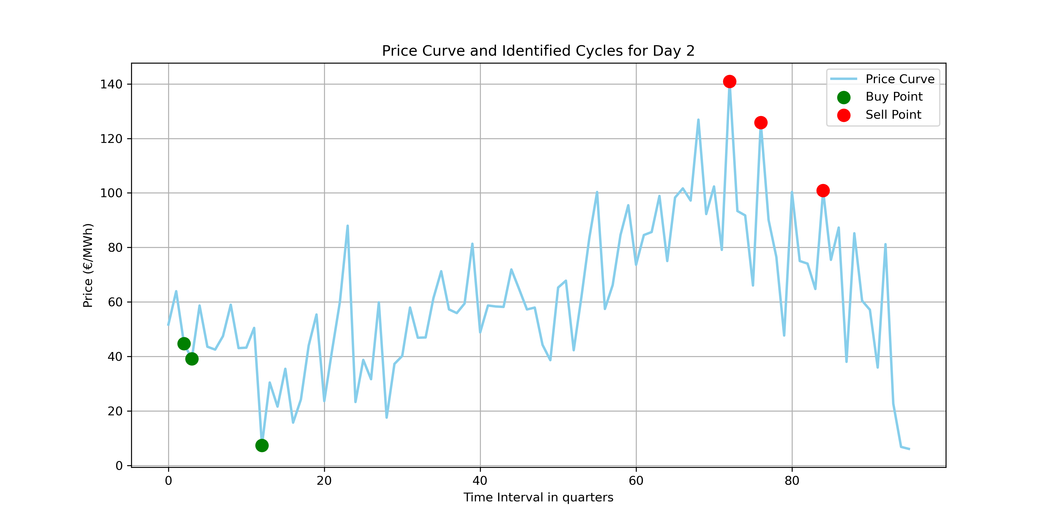
Price Curve and Identified Cycles for Day 2.
The second visualization is a bar chart that represents the cycle costs for the first 10 days of the dataset. Each bar corresponds to the net cost of cycling energy for a given day. The cycle costs are calculated by applying the estimate_cycle_costs function to the cycles identified by the calculate_daily_cycles function for each day’s price data.
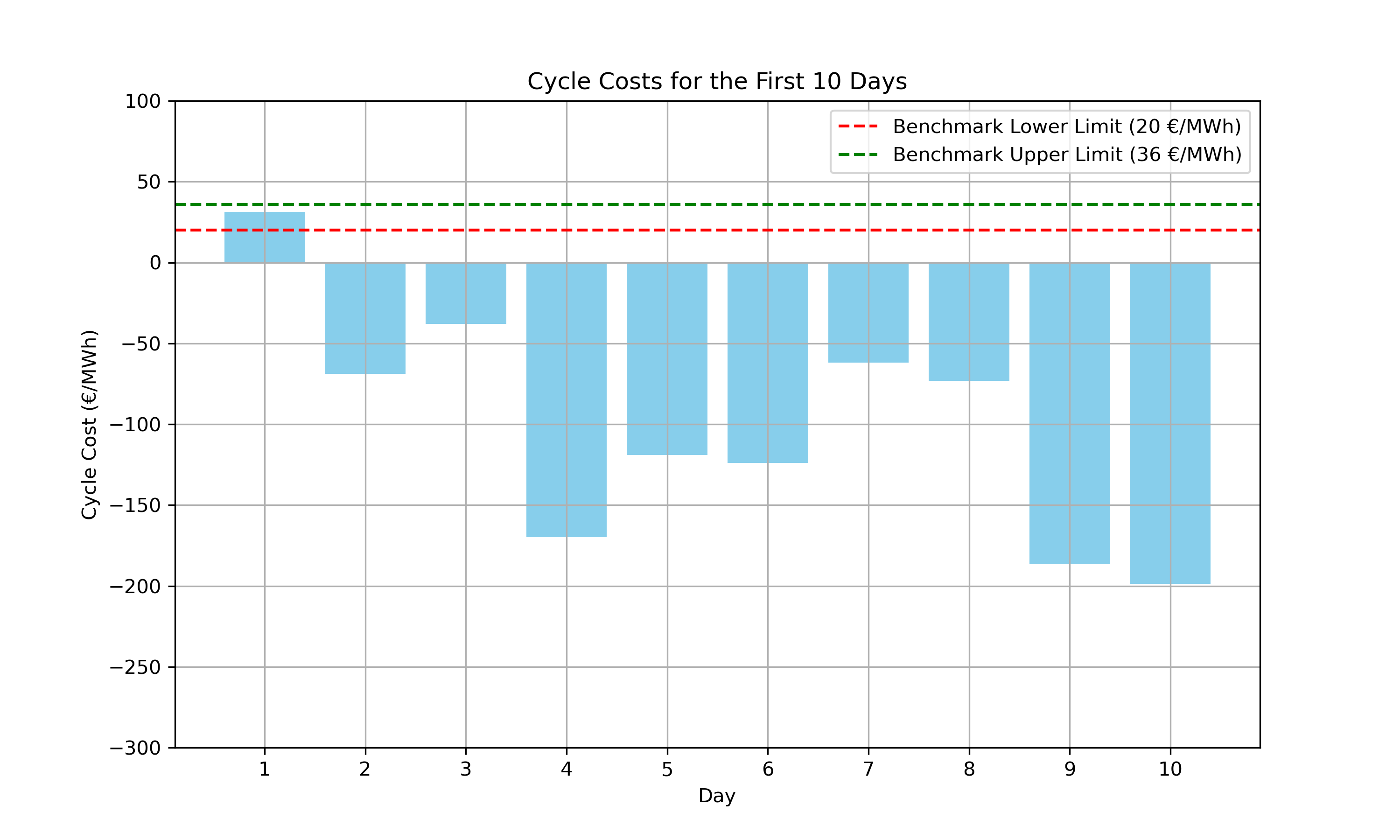
Cycle Costs for the First 10 Days.
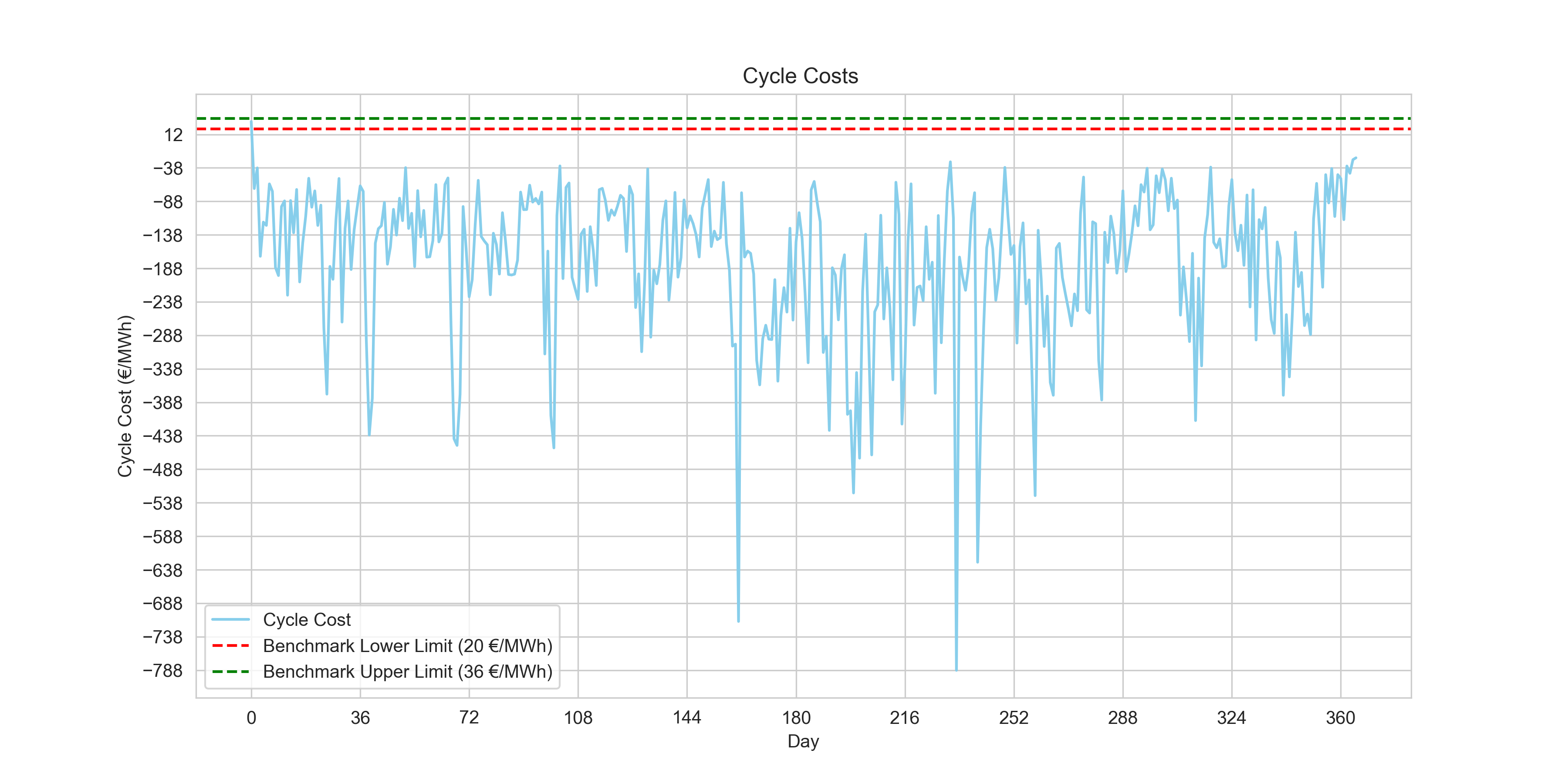
Cycle Costs for the entire dataset.
print(f"{((daily_price_data['cycle_cost'] >= 20) & (daily_price_data['cycle_cost'] <= 36)).sum()} day(s) within benchmark.")
Output
1 day(s) within benchmark.The first day showed cost results that within our benchmark. After examining the first day, there were only four data observations for the day. This reinforces the notion that a rolling horizon approach as the challenge also mentioned, might be a better method at identifying cycles within our benchmark
2. The Rolling Horizon Approach
Building upon the calculate_daily_cycles function, the rolling horizon approach introduces a more dynamic and responsive strategy. In the rolling horizon approach, instead of looking at the entire day’s data all at once, we analyze a smaller portion of data (a “window” of a few hours) and make decisions based on this smaller dataset. As we move through the day, this “window” rolls forward, giving us a new set of data to analyze.
The horizon length determines the size of the “window” of data that we are looking at during each step of the rolling horizon approach. The step size determines how much we move the horizon forward at each step. For example, with a step size of 4 intervals (representing 1 hour), after analyzing the first 3-hour window of data or horizon length (from time 0 to time 3 hours), we would move the window forward by 1 hour to analyze the next 3-hour window of data (from time 1 hour to time 4 hours). This means there would be a 2-hour overlap between consecutive windows.
1. Constructing the rolling horizon
def calculate_daily_cycles_rolling_horizonv2(price_data, current_avg_cycles, horizon_length=8, step_size=1):
    num_intervals = len(price_data)
    best_cycles = []

    #Dynamically change max number of cycles per day based on the target and current average number of cycles
    max_cycles_per_day = min(2.5, max(1, target_average_cycles + (target_average_cycles - current_avg_cycles)))
The code then dynamically adjusts the maximum number of cycles allowed each day. It calculates the difference between the target average cycles and the current average, using this information to modulate the daily cycle limit. This adjustment ensures that the algorithm progressively aligns with the target average, a crucial factor for long-term strategy implementation in fluctuating market conditions.
 # Loop over data with the rolling horizon
    for start_time in range(0, num_intervals, step_size):
        end_time = min(start_time + horizon_length, num_intervals)
        best_spreads = []
    return best_cycles
A new for loop iterates over the data in increments defined by ‘step_size’. For each iteration, it defines a ‘rolling horizon’ window, marked by ‘start_time’ and ‘end_time’. This window is where the algorithm searches for the most profitable trading cycles. By continuously moving this window across the dataset, the algorithm stays responsive to changing market conditions, ensuring that it captures the most advantageous trade opportunities as they arise. The code continues using the same combinatory logic of the previous approach.
The key component of optimizing the algorithm with the target average is creating a loop to dynamically adjust the maximum number of cycles per day based on the current average number of cycles and calculating the cycle cost for each day accordingly.
current_avg_cycles = 0
num_days = len(daily_price_data)

for i in range(num_days):
    daily_data = daily_price_data['EUR/MWh'].iloc[i]
    cycles = calculate_daily_cycles_rolling_horizonv2(daily_data, current_avg_cycles)
    cycle_cost = estimate_cycle_costs(cycles)
    daily_price_data.at[i, 'cycle_cost'] = cycle_cost
    current_avg_cycles = ((current_avg_cycles * i) + len(cycles)) / (i + 1)
The code begins by initializing current_avg_cycles at zero to represent the initial cycle count, and num_days determines the total days to iterate through. In each iteration of the loop, the daily price data is extracted and the calculate_daily_cycles_rolling_horizonv2 function computes the day’s cycles, taking into account the current average number of cycles. It then estimates the cycle cost using estimate_cycle_costs and updates this cost to the dataset. After each day’s calculation, the current average number of cycles is recalculated to include the latest data, ensuring that each new cycle count is informed by the most up-to-date average. In this way, the rolling horizon approach offers a significant enhancement over the static combinatory approach.
2. Identifying the best parameters
To improve the current strategy further, we embarked on a systematic exploration of different horizon lengths and step sizes. This experimentation involved running the rolling horizon function with various combinations of these two parameters to identify which horizon lengths and step sizes would yield the highest number of days with cycle costs within the benchmark.
#Trying out different parameters
results = []

for horizon_length in [4, 8, 12, 16, 20, 24, 28, 32]:
    for step_size in [1, 2, 4, 6, 8, 10]:
        daily_cycle_costs = daily_price_data['EUR/MWh'].apply(
            lambda x: estimate_cycle_costs(calculate_daily_cycles_rolling_horizon(x, horizon_length=horizon_length, step_size=step_size))
        )
        results.append({
            'horizon_length': horizon_length,
            'step_size': step_size,
            'days_within_benchmark': ((daily_cycle_costs >= 20) & (daily_cycle_costs <= 36)).sum()
        })

results_df = pd.DataFrame(results)
results_df.sort_values(by='days_within_benchmark',ascending=False).head()
Output
| horizon_length | step_size | days_within_benchmark |
|---|---|---|
| 8 | 1 | 90 |
| 8 | 2 | 90 |
| 8 | 4 | 89 |
| 8 | 6 | 89 |
| 8 | 10 | 89 |
The code iterates over a predefined set of horizon lengths and step sizes, applying each combination to the daily price data. For each set of parameters, it calculates the cycle costs for each day and then aggregates the number of days where the cycle cost falls within the benchmark range. With the horizon length of two hours and step sizes of 1 and 2 yielding the highest results, respectively.
3. 89 new observations within benchmarks
Upon visualizing the results, we get very favorable outcomes
plt.figure(figsize=(12, 6))

plt.plot(daily_price_data.index, daily_price_data['cycle_cost'], color='skyblue', label='Cycle Cost')
plt.axhline(y=20, color='r', linestyle='--', label='Benchmark Lower Limit (20 €/MWh)')
plt.axhline(y=36, color='g', linestyle='--', label='Benchmark Upper Limit (36 €/MWh)')
plt.xlabel('Day')
plt.ylabel('Cycle Cost (€/MWh)')
plt.title('Cycle Costs w/ Rolling Horizon')
plt.legend()
plt.grid(True)
plt.xticks(range(0, len(daily_price_data['cycle_cost']), int(len(daily_price_data['cycle_cost'])/10)))
plt.yticks(range(int(daily_price_data['cycle_cost'].min()), int(daily_price_data['cycle_cost'].max()), 50))
plt.show()
print(f"{((daily_price_data['cycle_cost'] >= 20) & (daily_price_data['cycle_cost'] <= 36)).sum()} day(s) within benchmark. \nCurrent Average Number of cycles: {round(current_avg_cycles, 3)}")
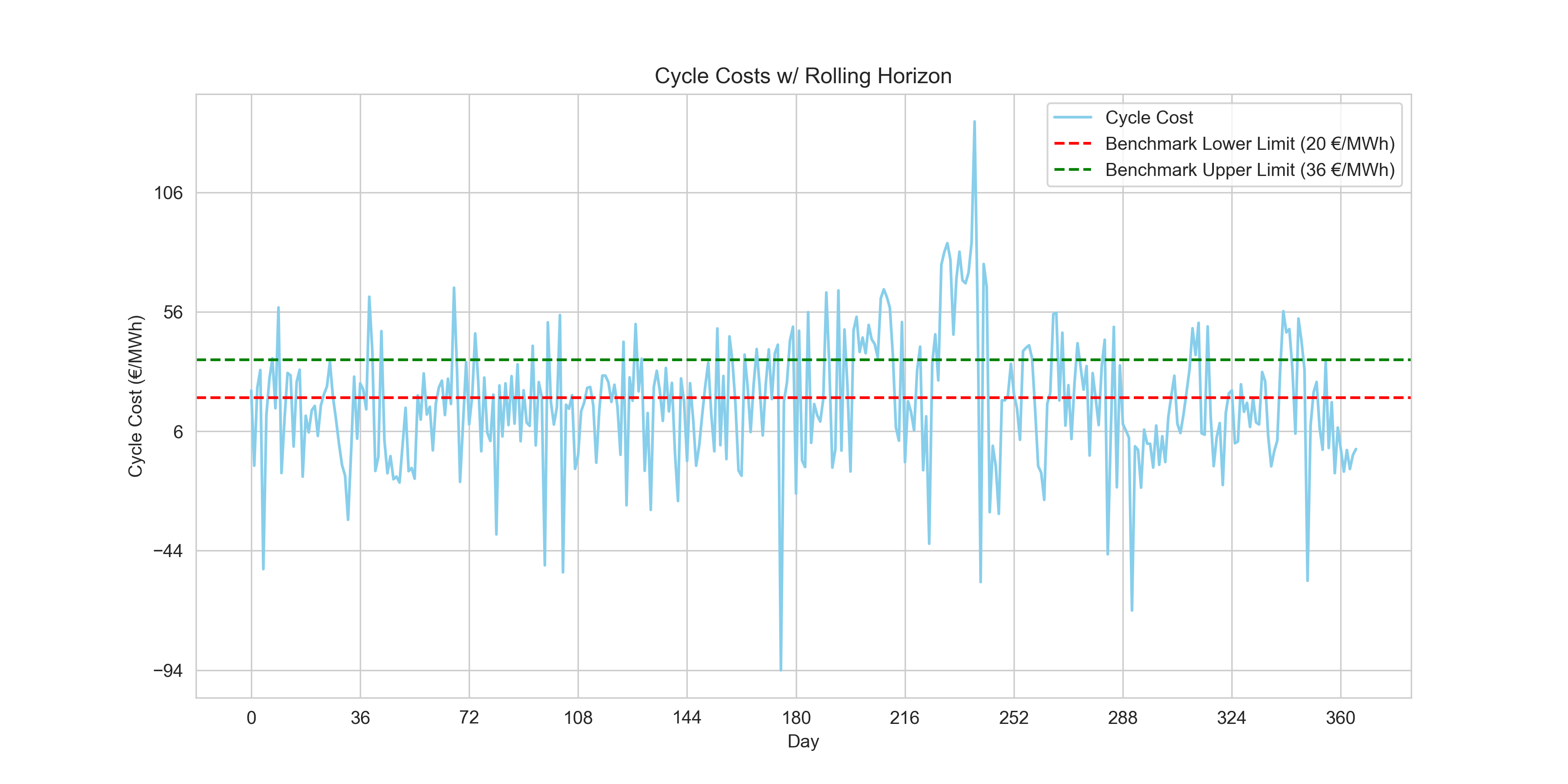
Cycle costs with rolling horizon approach.
Output
90 day(s) within benchmark.
Current Average Number of cycles: 1.997
The number of observations where the daily average cycle cost increased to 90 observations using the rolling horizon approach, indicating a significant improvement in the algorithm so far to meet benchmark criteria.
Upon examining the bar chart, we notice that the cycle costs vary across the days, with some days showing negative cycle costs, indicating profit, and others potentially indicating a loss if the costs were above zero. Although the vast majority of the cycle costs lie well below zero demonstrating that the algorithm is profitable, it is well below the benchmark range set by this challenge.
3. The Constrained Optimization Approach
Upon encountering this obstacle, I had to do some research on how to approach this project as my only data science experience so far was related to machine learning algorithms. On data science forums as I was debating my combinatory rolling horizon approach, it was pointed out to me that perhaps I’d find my answer in a constrained optimization approach. Although ignorant of it at first, I found it extremely fitting to the problem at hand! The approach attempts to identify the best ways to maximize a function within a set of hard and soft constraints. Sounds familiar?
It uses linear programming to maximize our energy trading strategy’s profitability. By utilizing the entire dataset from the outset, the optimization model takes a holistic view of the data, analyzes all these potential cycles collectively and determines the optimal set of cycles that could achieve the maximum possible profit. It compiles all possible trading cycles from the entire dataset of energy prices upfront. Each cycle’s profitability is assessed based on the prices at potential buy and sell times, factoring in the system’s operational constraints such as energy capacity, charging and discharging efficiencies, and the overall number of cycles allowed.
This approach contrasts with a rolling horizon, which would have looked at the data in chunks—optimizing over a short window and then rolling that window forward through the dataset, iteratively recalculating the optimal cycles as new price data becomes available.
Therefore, I chartered out to use a solver that makes use of SciPy, the famous Python package for mathematical computations among other uses.
1. Defining decision variables
This part of the code introduces the generate_possible_cycles function, which is designed to enumerate all possible buying and selling cycles for a single day’s worth of price data, called which will be used as the decision variables. This function is a critical component in constructing a constrained optimization approach, as it lays the groundwork for defining the decision variables. The function operates identically to the original function calculate_daily_cycles used in the combinatory approach, without the need to calculate and sort the best spreads separately, or break the function when it reaches the maximum number of cycles allowed.
#Create function to generate all possible cycles for one day, important for defining decision variable.
def generate_possible_cycles(price_data, min_length=1):
    num_intervals = len(price_data)
    possible_cycles = []

    for buy_time, sell_time in combinations(range(num_intervals), 2):
        if sell_time - buy_time >= min_length:
            spread =  (price_data[sell_time] * efficiency * efficiency) - price_data[buy_time]
            required_input_energy = capacity / efficiency
            bought_energy = min(nominal * (sell_time - buy_time) * 0.25, required_input_energy)
            charged_energy = bought_energy * efficiency
            discharge_energy = charged_energy * efficiency
            profit = price_data[sell_time]*discharge_energy -price_data[buy_time]*bought_energy

            possible_cycles.append({
                'buy_time': buy_time,
                'sell_time': sell_time,
                'bought_energy': bought_energy,
                'charged_energy': charged_energy,
                'discharge_energy': discharge_energy,
                'buy_price': price_data[buy_time],
                'sell_price': price_data[sell_time],
                'spread': spread,
                'profit': profit,
            })

    return possible_cycles


sample_day_data = daily_price_data['EUR/MWh'].iloc[1]
sample_possible_cycles = generate_possible_cycles(sample_day_data)
sample_possible_cycles_df = pd.DataFrame(sample_possible_cycles)
sample_possible_cycles_df.head()

#Create function to generate possible cycles for all days
def generate_possible_cycles_for_all_days(daily_price_data, min_length=1):
    all_possible_cycles = []

    for day_index, price_data in enumerate(daily_price_data['EUR/MWh']):
        daily_possible_cycles = generate_possible_cycles(price_data, min_length)

        #add day index to each cycle to identify the day to which it belongs
        for cycle in daily_possible_cycles:
            cycle['day_index'] = day_index

        all_possible_cycles.extend(daily_possible_cycles)

    return all_possible_cycles

all_possible_cycles = generate_possible_cycles_for_all_days(daily_price_data)
all_possible_cycles_df = pd.DataFrame(all_possible_cycles)
all_possible_cycles_df.head(), all_possible_cycles_df.info()
Output
<class 'pandas.core.frame.DataFrame'>
RangeIndex: 1664032 entries, 0 to 1664031
Data columns (total 10 columns):
 #   Column            Non-Null Count    Dtype
---  ------            --------------    -----
 0   buy_time          1664032 non-null  int64
 1   sell_time         1664032 non-null  int64
 2   bought_energy     1664032 non-null  float64
 3   charged_energy    1664032 non-null  float64
 4   discharge_energy  1664032 non-null  float64
 5   buy_price         1664032 non-null  float64
 6   sell_price        1664032 non-null  float64
 7   spread            1664032 non-null  float64
 8   profit            1664032 non-null  float64
 9   day_index         1664032 non-null  int64
dtypes: float64(7), int64(3)
memory usage: 127.0 MB
The results show over 1.66 million possible cycles, validating the success of this step.
2. Using linear programming
Linear programming is a powerful tool used in operations research to find the best outcome in a mathematical model whose requirements are represented by linear relationships. In the context of our project, LP will help us identify the most profitable set of cycles that can be executed within the operational constraints of the energy storage system.
The days_number variable represents the total number of days in our dataset. We then extract the profits from all possible cycles and create an objective function, c, which is the negation of the profits because LP minimizes the objective function by default, and we are aiming to maximize profits.
To ensure that our solution adheres to the operational constraints, we introduce A_eq_daily, a matrix that creates equality constraints to limit the number of cycles executed each day to a maximum of max_cycles_per_day. Additionally, we enforce the target average number of cycles across all days by setting up A_eq_average.
#Using linear programming
days_number = daily_price_data.shape[0]

profits = all_possible_cycles_df['profit'].values
day_indices = all_possible_cycles_df['day_index'].values
c = -profits
lambda_penalty = 1e6

A_eq_daily = np.zeros((days_number, len(profits)))
for i in range(days_number):
    A_eq_daily[i, day_indices == i] = 1

A_eq_average = np.ones((1, len(profits)))

A_eq = np.vstack([A_eq_daily, A_eq_average])
b_eq = np.hstack([np.full(days_number, max_cycles_per_day), [target_average_cycles * days_number]])

c_extended = np.append(c, lambda_penalty)#Extend c to account for the penalty on the deviation variable delta


A_eq_delta = np.append(np.ones(len(profits)), [-1]).reshape(1, -1)
A_eq = np.hstack([A_eq, np.zeros((A_eq.shape[0], 1))])  # Add a column for delta to A_eq
A_eq[-1, :] = A_eq_delta  # Update the last row with A_eq_delta


bounds = [(0, 1) for _ in profits] + [(0, None)]
print(A_eq.shape, b_eq.shape)
We stack these constraints together in A_eq and combine them with b_eq, which is the array of values that our equality constraints must equal. We include the target average multiplied by the number of days as part of b_eq to enforce our average cycling target over the entire period.
The problem complexity increases as we introduce lambda_penalty, a large penalty for deviation from our target average cycle count. This is a common approach in LP to strongly discourage the solution from straying from this target. We extend our cost vector c to include this penalty factor.
To account for this penalty in our constraints, we expand A_eq to include an additional column for the penalty variable, delta, which represents the deviation from the average cycle target. This ensures that any deviation is heavily penalized in the objective function, pushing the LP solution towards our desired average.
The bounds ensure that our decision variables, which represent whether or not to execute a given cycle, are either 0 or 1, effectively making this a binary decision. We also allow the penalty variable, delta, to be greater than or equal to zero, indicating that it can adjust freely to reflect any deviation from the target average.
Finally, we print the shapes of A_eq and b_eq to verify that our constraints are correctly dimensioned for the LP solver.
Output
(367, 1664033) (367,)
2.1 Using the solver
res_option_b = linprog(c_extended, A_eq=A_eq, b_eq=b_eq, bounds=bounds, method='highs')
print(res_option_b)
message: Optimization terminated successfully.
            (HiGHS Status 7: Optimal)
success: True
    status: 0
    fun: 365095106.33555603
        x: [ 0.000e+00  0.000e+00 ...  0.000e+00  3.660e+02]
    nit: 375
    lower:  residual: [ 0.000e+00  0.000e+00 ...  0.000e+00
                        3.660e+02]
            marginals: [ 1.707e+01  4.832e+01 ...  1.425e+02
                        0.000e+00]
    upper:  residual: [ 1.000e+00  1.000e+00 ...  1.000e+00
                            inf]
            marginals: [ 0.000e+00  0.000e+00 ...  0.000e+00
                        0.000e+00]
    eqlin:  residual: [ 0.000e+00  0.000e+00 ...  0.000e+00
                        0.000e+00]
            marginals: [ 1.000e+06  9.996e+05 ...  9.999e+05
                        -1.000e+06]
ineqlin:  residual: []
            marginals: []
 mip_node_count: 0
 mip_dual_bound: 0.0
        mip_gap: 0.0
By implementing the linear programming solver with our defined objective function and constraints, we have calculated the most profitable set of energy trades while respecting the operational constraints of our system. The solver’s output provides several pieces of crucial information:
The objective function value (fun) represents the total profit from the selected cycles under the optimal solution. This figure is the maximized profit, considering the costs and constraints in our model. The variable X includes the decision variables for each potential cycle, indicating which cycles are to be executed to achieve the optimal profit. The mip_gap shows that the solution is optimal since its value is 0. This means there is no gap between the best-known solution and the worst-case bound on the objective function, underscoring that the optimal solution is indeed the best possible under the given model.
x_values = res_option_b['x'][:-1]
suggested_cycle_indexes = np.where(x_values == 1)[0]
suggested_cycles_df = all_possible_cycles_df.iloc[suggested_cycle_indexes]
suggested_cycles_df
We construct a Dataframe with the selected cycles. The ‘x_values’ extracted from the res_option_b output represent the binary decisions for each possible cycle—whether a cycle should be executed (1) or not (0). By isolating these decision variables, we can pinpoint exactly which cycles the optimization model has determined to be the most profitable within the constraints.
Using a simple condition to locate where x_values equals 1, we identify the indices of the suggested cycles. These indices correspond to the rows in our all_possible_cycles_df DataFrame that the optimization model has selected.
The DataFrame suggested_cycles_df is then created by filtering all_possible_cycles_df with the suggested cycle indices. This DataFrame is a subset of the original and contains only the cycles that our LP model recommends for execution. It provides all the necessary details of each recommended cycle, such as the buy and sell times, energy amounts at each stage, and the expected profit.
suggested_df = suggested_cycles_df.groupby('day_index').apply(lambda x: x.to_dict('records'))The suggested_cycles_df was restructured using the groupby method to aggregate cycles by day. The apply method was then used with a lambda function to convert each group into a dictionary of records. This transformation was necessary to align the data with the input requirements of the estimate_cycle_costs function, which we defined earlier in the project. This function calculates the net cost or profit of executing a series of cycles throughout a day.
3. Visualizing the suggested cycles
#Plotting out final cycle cost estimations using the suggest cycles of the linear programming method.
daily_price_data['cycle_cost'] = suggested_df.apply(estimate_cycle_costs)

plt.figure(figsize=(12, 6))

plt.plot(daily_price_data.index, daily_price_data['cycle_cost'], color='skyblue', label='Cycle Cost')
plt.axhline(y=20, color='r', linestyle='--', label='Benchmark Lower Limit (20 €/MWh)')
plt.axhline(y=36, color='g', linestyle='--', label='Benchmark Upper Limit (36 €/MWh)')
plt.xlabel('Day')
plt.ylabel('Cycle Cost (€/MWh)')
plt.title('Cycle Costs of Suggested Cycles w/ Constrained Optimization Approach')
plt.legend()
plt.grid(True)
plt.xticks(range(0, len(daily_price_data['cycle_cost']), int(len(daily_price_data['cycle_cost'])/10)))
plt.yticks(range(int(daily_price_data['cycle_cost'].min()), int(daily_price_data['cycle_cost'].max()), 50))
plt.show()

print(f"{((daily_price_data['cycle_cost'] >= 20) & (daily_price_data['cycle_cost'] <= 36)).sum()} day(s) within benchmark.")
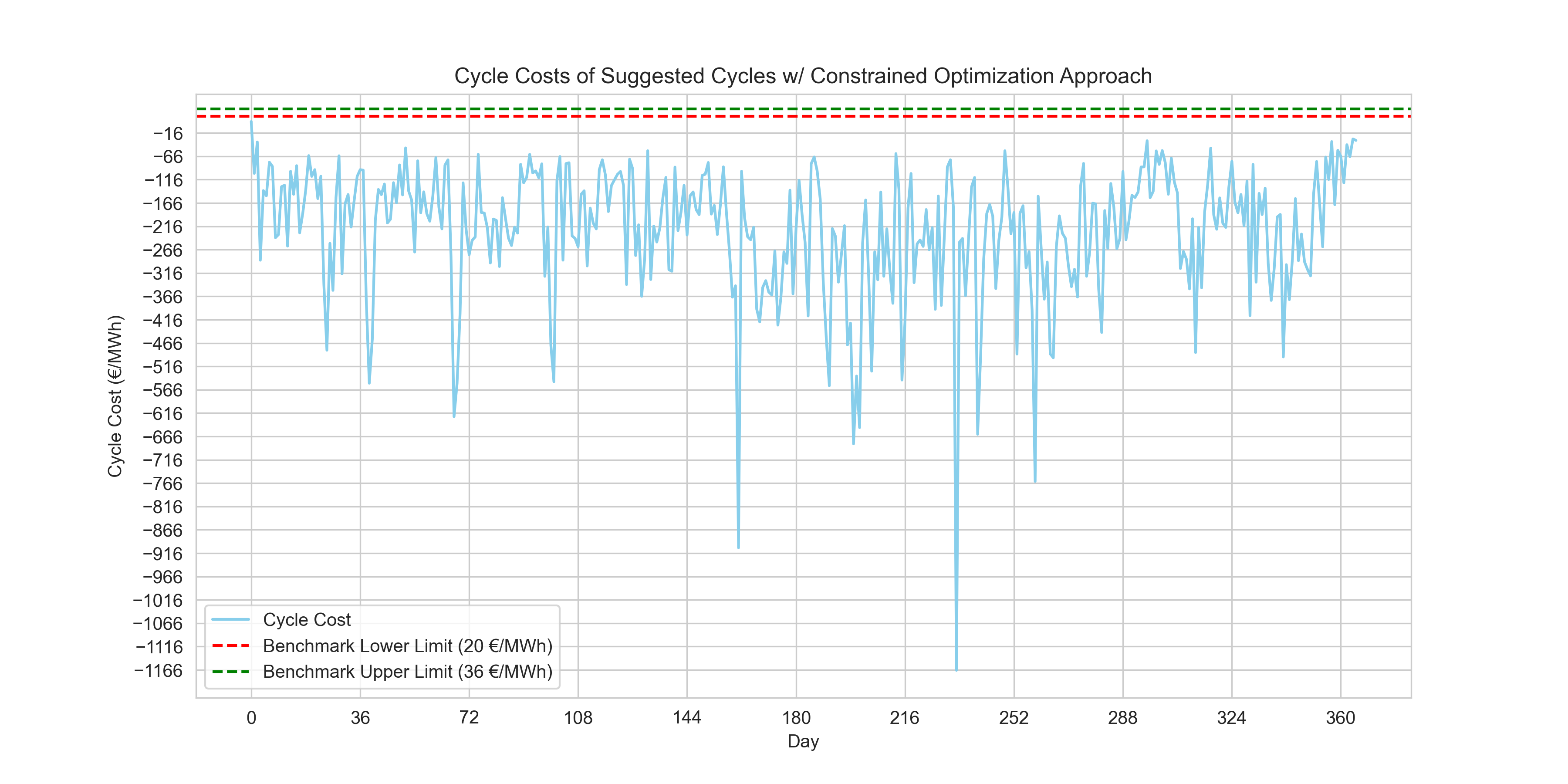
Cycle costs per day of the suggested cycles by the linear programming solver.
Output
0 day(s) within benchmark.Conclusion
The results from the constrained optimization approach showed the cycle costs of the suggested cycles per day yielded no days within the benchmark. The benchmark costs are still unexplained from my side as it relates to this challenge; why are they in the positive range if the purpose of every cycle is to generate a profit i.e. a figure within the negative range.
Putting the benchmarks aside for a second and focusing solely on profit maximization, we proceed to compare the total cycle costs—or in this context, the total profits—generated by each approach.
print(f"Total costs of selected cycles with the Combinatory ArpprApproachoach:\n{daily_price_data['EUR/MWh'].apply(lambda x:estimate_cycle_costs(calculate_daily_cycles(x))).sum()}\n")
print(f"Total costs of selected cycles with the Rolling Horizon Approach:\n{daily_price_data['EUR/MWh'].apply(lambda x:estimate_cycle_costs(calculate_daily_cycles_rolling_horizonv2(x, 0))).sum()}\n")
print(f"Total costs of selected cycles with the Constrained Optimization Approach:\n{suggested_df.apply(estimate_cycle_costs).sum()}\n")
Output
Total costs of selected cycles with the Combinatory Approach:
-65250.43239985398

Total costs of selected cycles with the Rolling Horizon Approach:
8673.51469943505

Total costs of selected cycles with the Constrained Optimization Approach:
-82084.92143421053
The results indicate that for the:
- Combinatory Approach: The negative sum suggests that this approach, overall, has resulted in a significant profit when considering all selected cycles across the dataset.
- Rolling Horizon Approach: The positive sum here is unexpected, as we're looking to maximize profit. This might indicate that the selected cycles did not perform as well, or perhaps there is a need to revisit the implementation of this approach, as typically we would expect this to be a negative value denoting profit.
- Constrained Optimization Approach: The approach appears to have yielded the highest profit as indicated by the most negative sum, suggesting that when it comes to total profit across all cycles, this approach was the most effective.
In summary, my exploration into algorithmic trading through the lens of energy storage systems revealed the constrained optimization approach as the standout strategy for maximizing profits. While the results are promising, they also pave the way for further refinement. Understanding the benchmark costs in greater depth and investigating the potential of Mixed-Integer Linear Programming to manage overlapping cycles are immediate next steps.
The project so far represents Version 1 of my solution and is bound to be revisited again. The full project and data are available on my GitHub.